In 1809, on a battlefield in Portugal, the first recognisable medical trial evaluated bloodletting on a sample of 366 soldiers allocated into treatment and control groups. The cure was shown to be bogus. It was the beginning of the end of pre-modern medicine. Yet problems of allocation bias— i.e., ‘insufficient randomisation’ – pervaded poor experimental designs until the landmark British Medical Research Council trials of patulin and streptomycin in the 1940s. Since then the randomised controlled trial has been the foundation of evidence-based medicine.
Is a similar evidence-based macroeconomics possible? One pressing and highly topical context is the effects of austerity on output (see Alesina and Ardagna 2010, Guajardo et al. 2011). This might seem like a natural and helpful line of debate. Natural, since experimental techniques drawn from medicine have been fruitfully incorporated in other fields of economics. Helpful, for some, since more clarity on fiscal impacts might be welcome, given the uproar over European and UK austerity programs.
Ironically, the policy debate is sprinkled with medical metaphors. In 2011 German Finance Minister Wolfgang Schäuble wrote that “austerity is the only cure for the Eurozone”; while Paul Krugman likened it to “economic bloodletting”. In the Financial Times, Martin Wolf, cautioned that “the idea that treatment is right irrespective of what happens to the patient falls into the realm of witch-doctoring, not science” while Martin Taylor, former head of Barclays, put it quite bluntly: “Countries are being enrolled, like it or not, in the economic equivalent of clinical trials.”1
In a new paper we exploit a treatment-control design using statistical techniques designed for situations, experimental or otherwise, where underlying allocation bias may prevail (Jordà and Taylor 2013). This turns out to be a serious problem here, as in many other macroeconomic contexts where endogenous policy actions epitomise the “insufficient randomisation” problem.
Confronting the great austerity debate
For consistency we use the very same OECD annual panel dataset (17 economies; 1978–2009) common to two high-profile yet contradictory studies. The influential “expansionary austerity” idea came to be associated with Alesina and Ardagna (2010); but an IMF study reached the opposite conclusion of “contractionary austerity” (Guajardo et al. 2011).
For minimal parameterisation, we use local projection methods (Jordà 2005) to estimate output impacts of fiscal policy up to four years out. These flexible methods permit us to compare different identification strategies and easily allow for possibly non-linear, or state-dependent responses. Indeed we find that responses are very different in booms and slumps, as emphasised by Keynes in the 1930s.
Step 1: Replicating expansionary austerity
The simplest identification of the causal effect of a fiscal policy intervention relies on a weak form of the selection-on-observables assumption. Conditional on a set of controls, variation in policy interventions is supposedly largely random. However, if policy interventions conditional on controls are systematically determined by an unobserved variable that is correlated with the outcome then the method fails.
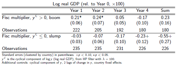
As a first step we estimate linear-projection impacts of fiscal policy using the Alesina-Ardagna measure of policy, the change in the cyclically-adjusted primary balance from year 0 to year 1.2 These first estimates suggest, consistent with Alesina-Ardagna, that austerity is expansionary. The significant coefficients here have a positive sign. In Table 1 we stratify the results by the state of the cycle (2 bins, boom and slump, based on the sign of HP-filtered log output, yC) at time 0; we see that the result is entirely driven by what happens in booms. It is only in booms that we find a significant response of real GDP to fiscal tightening, with a coefficient or multiplier of about +0.2* in years 1 and 2 (+ p < 0.10, * p < 0.05). The effects seem to taper off in years 3 and 4. But in slumps, the policy response is not statistically significant and is typically negative.
Table 1. Estimates of the impact of 1% of GDP fiscal consolidation, by state of the economy
Step 2: Replicating contractionary austerity
Alternative identification is possible if valid instrumental variables are available. This method assumes that if there is correlation between the instrument and the control, then one has a source of exogenous variation in policy interventions with which to calculate the causal effect (e.g., Auerbach and Gorodnichecko 2013, Owyang et al. 2013).
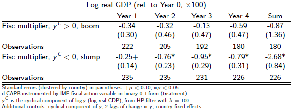
As a next step we therefore replace our linear-projection estimator with an instrumental-variable linear-projection estimator. The change in cyclically-adjusted primary balance is instrumented by the IMF set of potential ‘narrative’ instruments, i.e. indicators of dates of fiscal consolidations that, through a reading of the historical record, might be reasonably considered to be exogenous.3 Here the findings are very much consistent with the IMF results in Table 2.
Austerity appears contractionary. The significant coefficients here have a negative sign. However, stratification shows that this result is now largely driven by what happens in slumps. The effects in a boom are imprecisely estimated but negative. In a slump we find significant negative responses of real GDP to fiscal tightening from year 1 all the way out to year 4. Over 4 years the sum of these effects is −2.68*, so the average loss for a 1% of GDP fiscal consolidation is a depressed output level of about to 0.7% per year over this horizon.
Table 2. Instrumental-variable estimates of the impact of 1% of GDP of fiscal consolidation, by state of the economy
Endogenous austerity: The fiscal treatment is not randomly allocated
Naturally, a key question is whether these instruments are really exogenous. In fact, they aren’t. The IMF’s fiscal consolidation episodes can be predicted using predetermined macroeconomic controls. They may not be valid instruments. Thus, even with this instrument, which might alleviate the most glaring issues of endogeneity and measurement bias, some endogeneity remains in the treatment variable.
We find evidence here from multiple criteria, including exogeneity tests and balance checks. Table 3 presents probit models of the IMF treatment variable (a consolidation from year 0 to year 1). In column 1 the austerity treatment is more likely when public debt is higher. Governments pursue austerity when debt is elevated. In column 2, when output is further below potential or growing more slowly, there is an increase in the likelihood of treatment. Finally, columns 3 and 4 add the lag of treatment. Being in treatment today is a good predictor of being in treatment tomorrow. Austerity programs persist.
Table 3. Austerity treatment episodes are a non-random allocation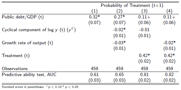
Step 3: Estimates of the average effect of fiscal consolidations
We offer a new take in a third and final step. If the IMF’s austerity treatment variable has a significant forecastable component this could induce allocation bias in estimated responses. To address this we use local projections again, but with an inverse probability weight regression-adjustment method to calculate average treatment effects.4
The inverse probability weight regression-adjustment estimator uses a saturated first-stage probit model to predict treatment probability based on observables, getting as close as possible to a quasi-randomised experiment. This first stage prediction is called the policy propensity score. The second stage outcome regression then corrects for the allocation bias in situations where the outcome also depends on observables, but is in every other respect exactly the same specification used in the linear-projection specifications. The consistency of this estimator is ‘doubly robust’ (unlike inverse probability weight or regression adjustment alone) and guards against incorrect model specification in either the treatment regression or the outcome regression.
Using the two-stage estimator, Table 4 shows that austerity has a mostly negative effect, all years, in both bins. It has larger and more statistically significant negative effects in the slump. In booms, which one could view as the ‘full employment’ case, we find smaller (and mostly statistically insignificant) impacts of fiscal consolidation on output. Summed over four years, the estimates of the average treatment effects are -1.13+ in booms but -2.48* in slumps.
Table 4. Doubly robust estimates of the impact of fiscal ‘treatment’, by state of the economy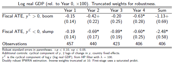
Three views of austerity: The good, the bad and the ugly
Our results contrast with the expansionary austerity view of Alesina and Ardagna, and even amplify the opposing view of the IMF. For comparisons we have to adjust for the scale of the treatments by the average treatment size, the mean of the IMF measured consolidation (in % of GDP). There is little variation in treatment size across the bins, so the average treatment effects are in fact comparable to multipliers because the average treatment, coincidentally and conveniently, is close to one.
In recent times austerity has been systematically applied in weak economic conditions: plus ça change. But in a bad current state the economy is more likely to grow faster than trend going forward. By failing to allow for the endogeneity of treatment we could end up with a far too rosy view of the aftermath of fiscal consolidations. A dead cat bounces, regardless of whether it jumped or was pushed.
Using ordinary-least-squares estimation we would walk away believing in expansionary austerity, or no effect when the economy is weak. Using ‘narrative’ instrument variables we might believe in contractionary austerity except when the economy is strong, but the estimates are possibly biased as the instruments may not be valid as allocation into treatment is not random. Using our two-stage method to deal with allocation bias, we find stronger evidence of contractionary austerity in the weak economy with much more precise estimates. These results suggest that only a strong economy can bear a fiscal consolidation without significant output losses.
Counterfactual: Coalition austerity and the UK recession
To provide illustration, we apply our estimates to make an (out-of-sample) counterfactual forecast of the post-2007 path of the UK economy without the fiscal austerity policies imposed by the coalition government after the 2010 election.
Two assumptions may be needed to make this exercise relevant. First, we assume that the UK had fiscal space and was not forced to do austerity; this may be defended in that real GDP is now worse than was expected in 2010, and debt to GDP higher than expected, yet gilt yields remain ultra-low in real terms (and at their lowest nominal level in their 280 years of recorded history). Second, we assume that policymakers care about timing fiscal adjustments so as to mitigate damage to the real GDP path of the economy; this is, at least, an oft-stated goal of most policymakers. The results are presented in Figure 1, where we show actual and forecast paths for UK real GDP from 2007 (the business cycle peak) through 2013. How much of the poorer outturn can be attributed to the fiscal policy choice of instigating austerity during a bad slump? The answer, using our model as described above, is about 60%. Without austerity, UK real output would now be steadily climbing above its 2007 peak, rather than being stuck 2% below.
Figure 1. UK actual path and counterfactual path without austerity
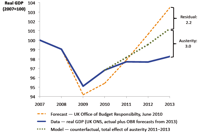
The residual relative to the forecast could be accounted for by various omitted factors, as has been noted (Davies 2012), such as export patterns in the Eurozone and idiosyncratic UK sector shocks. There could also have been over-optimism in the 2010 forecast. However, a major caveat suggests that we likely have a biased underestimate of the effects of current UK austerity. This caveat is the zero lower bound, when fiscal multipliers are known to be much larger in both theory and evidence. Our UK out-of-sample counterfactual does correspond to a ‘liquidity trap’ environment, but our in-sample data overwhelmingly do not.5 Thus our estimate of austerity’s effects in the UK is probably conservative.
Summary
Few economic policy issues generate as much controversy as the ongoing austerity argument, and, as Europe and the UK endure double-dip stagnation, the debate is probably far from over.
Fiscal consolidations are not exogenous events, even those identified by the narrative approach. By reweighting observational data to approximate an experiment where treatment is ‘as if’ at random (based on a first-stage model), we estimate policy responses in a way that corrects for allocation bias.
Our estimates are closer to those from the instrumental-variable specification than from the ordinary-least-squares specification. We confirm adverse impacts as in the IMF study. But we also find that this is a ‘bad times’ result. Fiscal contraction prolongs the pain when the state of the economy is weak, much less so when the economy is strong.
Keynes is still right, after all: “The boom, not the slump, is the right time for austerity at the Treasury.”
References
Alesina, A, and R Perotti (1995), “Fiscal Expansions and Adjustments in OECD Economies”, Economic Policy 10 (21): 207–247.
Alesina, A, and S Ardagna. (2010), “Large Changes in Fiscal Policy: Taxes versus Spending” In Tax Policy and the Economy, edited by J R Brown, vol. 24. Chicago: University of Chicago Press, pp. 35–68.
Almunia M, A Bénétrix, B Eichengreen, K H O’Rourke, and G Rua (2010), “From Great Depression to Great Credit Crisis: Similarities, Differences and Lessons”, Economic Policy 25 (62): 219–265.
Angrist, J D, Ò Jordà and G M Kuersteiner (2013), “Semiparametric Estimates of Monetary Policy Effects Before and Since the Great Recession: String Theory Revisited”, Paper presented at the NBER Summer Institute.
Auerbach, A J and Y Gorodnichenko (2013), “Fiscal Multipliers in Recession and Expansion”, In Fiscal Policy after the Financial Crisis edited by AAlesina and F Giavazzi. Chicago: University of Chicago Press.
Christiano L, M Eichenbaum and S Rebelo (2011), “When Is the Government Spending Multiplier Large?” Journal of Political Economy 119 (1): 78–121.
Davies, G (2012), “Why is the UK Recovery Weaker than the US?” Financial Times, November 14.
Eggertsson, G B, and P Krugman. (2012), “Debt, Deleveraging, and the Liquidity Trap: A Fisher-Minsky-Koo Approach”, Quarterly Journal of Economics 127 (3): 1469–1513.
Guajardo J, D Leigh, and A Pescatori (2011), “Expansionary Austerity: New International Evidence”, IMF Working Paper 11/158.
Hirano K, G W Imbens, and G Ridder (2003), “Efficient Estimation of Average Treatment Effects Using the Estimated Propensity Score”, Econometrica 71(4): 1161–1189.
Imbens, G W (2004), “Nonparametric Estimation of Average Treatment Effects Under Exogeneity: A Review”, Review of Economics and Statistics 86(1): 4–29.
Jordà, Ò and A M Taylor (2013), “The Time for Austerity: Estimating the Average Treatment Effect of Fiscal Policy”, Paper presented at the NBER Summer Institute.
Lunceford, J K and M Davidian (2004), “Stratification and weighting via the propensity score in estimation of causal treatment effects: A comparative study”, Statistics in Medicine 23: 2937–60.
Owyang M T, V A Ramey and S Zubairy (2013), “Are Government Spending Multipliers Greater During Periods of Slack? Evidence from 20th Century Historical Data”, NBER Working Paper 18769.
Rendahl, P (2012), “Fiscal Policy in an Unemployment Crisis”, Cambridge Working Papers in Economics 1211.
Robins, J M, A Rotnitzky and L P Zhao (1994), “Estimation of Regression Coefficients When Some Regressors are not Always Observed”, Journal of the American Statistical Association 89(427): 846–66.
Romer, C D, and D H Romer (1989), Does monetary policy matter? A New Test in the Spirit of Friedman and Schwartz. In NBER Macroeconomics Annual 1989 edited by Oliver J. Blanchard and Stanley Fischer. Cambridge, Mass.: MIT Press, pp. 121–170.
Footnotes
1 The quotes are from ft.com, nytimes.com, ft.com and ft.com, respectively.
2 We can consider all such shocks, or restrict attention to “large” shocks (larger in magnitude than 1.5% of GDP), a cutoff value used by Alesina and Ardagna and proposed earlier by Alesina and Perotti (1995), but the results are robust to these changes.
3 This is “narrative-based identification” (e.g. Romer and Romer 1989).
4 On the inverse-probability-weight estimator in economics see Hirano etal. (2003); for an application to macroeconomics with policy propensity scores, see Angrist et al. (2013). On the inverse probability weight regression-adjustment estimator and the “doubly robust” property see Robins et al. (1994) and Lunceford and Davidian (2004). A survey of these and related estimators is found in Imbens (2004).
5 Our estimates are based on a sample from 1978 to 2007, when the zero lower bound was virtually absent from any country-year observations in the dataset (the only exceptions being 7 country-year observations, out of a total of 173 consolidation episodes, all of these relating to Japan in the 1990–2007 period). As is well known in theory (Christiano et al. 2011; Eggertsson and Krugman 2012; Rendahl 2012) and also from historical evidence from the Great Depression (Almunia et al. 2010), fiscal multipliers are much larger in zero-lower-bound conditions than in normal times when monetary policy is away from this constraint. But in the post-2008 forecast period for the UK the zero lower bound was a binding constraint, which would tend to make even our already large estimated fiscal impacts an underestimate of the true impacts.


