Rising unemployment due to the pandemic lockdown will mean higher profits for many businesses, as they generate savings due to a lower wage bill and higher productivity, despite reduced economic activity. These savings, together with previously undistributed corporate profits, enable corporations to lend to the federal government so it can finance its current deficit-spending spree. The surge in profits benefits high-income households who trade in government bonds. In other words, the government’s efforts to combat the COVID-19 economic crisis ultimately creates wealth in the form of Treasury bonds for households at the top.
Double-entry bookkeeping, with debits in one account financed by credits from others, has been around for a couple thousand years. In America now, credit and debit arithmetic is crucial to understanding how massive short-run fiscal outlays to combat the COVID-19 pandemic will be financed. Details emerge from double entries built into the national income accounts invented 80 years ago by John Maynard Keynes and others (Taylor, 2010). The bottom line is that lending from corporations’ undistributed profits (one-third of new government debits) and households (most of the rest) will be required. Much of the household net lending or saving less capital formation will be provided by the top 1% who benefit disproportionately from distributed profit income.
Before looking at the background since the Great Recession a decade ago and the current numbers, key observations are the following:
1) The consolidated government deficit (Federal, State, and local) is likely to rise this year by at least three trillion dollars, or 15% of GDP (Taylor, 2020). To attain macroeconomic balance this debit item (or government net borrowing) will have to be funded by credits from corporate business, households, and the rest of the world – there are no other sources. Business and household credits are created by higher incomes than spending flows; foreign credits pay for greater imports than exports.
2) The force driving business profits will be productivity growth. In this year’s second quarter, forecasts suggest that real output will fall by several percentage points. Employment will drop from its level in March by even more. Labor productivity or the ratio of output to employment will increase. Income generated by production mostly takes the form of payments to labor and profits. If wages are relatively flat, higher productivity implies that the profit share of income will rise, increasing business saving. In the short run at least, these enhanced retained earnings will help pay for new government net borrowing.
3) Households, meanwhile, already increased their savings in the first quarter, and outstanding consumer credit fell by 20% (at an annual rate) in April.[1] A second quarter increase in net lending is a likely continuation of these trends. Households in the top one percent of the size distribution of income receive the bulk of non-retained business earnings. They also get capital gains, which average out approximately to equal undistributed corporate profits (Taylor with Ömer, 2020).
An old post-Keynesian adage (probably due to Nicholas Kaldor or Joan Robinson and often associated with Michal Kalecki) states that “Capitalists earn what they spend, workers spend what they earn.” Under present circumstances it might be restated as “Government borrows what it doesn’t tax, corporations and rich households gain wealth by lending to government profit income they don’t spend.”
Historical record
The aim of this year’s surge in government net borrowing is to stimulate aggregate demand, generating output and putting people back to work. Similar policies were applied after the financial crisis a dozen years ago. Figure 1 shows how sectoral debit and credit flows responded. (Net borrowing shares of GDP are shown as positive because they add to effective demand.)
In the years just before the crisis, government net borrowing was largely financed by new loans from abroad (the famous twin deficits). When the 2007-09 recession struck, it was precipitated by private sector retrenchment. Household consumption was flat, while gross business investment fell by 30%. Household saving and business retained earnings went up, meaning that the overall private saving share of GDP rose from 19% to 22%.
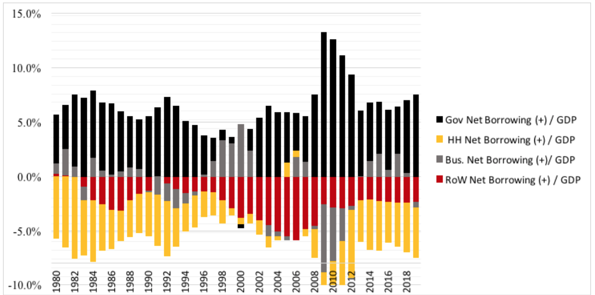
Figure 1: Annual sectoral net borrowing shares of GDP
Output actually increased between 2007 and 2009. It would have dropped dramatically if the GDP share of government taxes minus transfers to households had been stable. But in fact it fell from 15% to 6% due to automatic stabilizers and the Obama stimulus package of around 5% of GDP. The overall impact was that private net
borrowing fell by 10.2% of output while government borrowing went up by 8.6%. Reduction of the external deficit by 1.7% made up the difference.
Higher business net lending (think of that as negative net borrowing) took the lead in financing government debits in 2009-10. Thereafter through 2019, households were the main source of funds, as their savings share of GDP went up.
Current economic predictions are dire. In the first quarter the pandemic forced massive business closures and job losses. How will credits from business, households, and the rest of the world bankroll massive government intervention? Given its importance in Figure 1, we can begin with business net lending.
Can corporate net lending finance the fiscal deficit?
The drop in real gross domestic product (GDP) during the second quarter may be in the range of six percent.[2] The ratio of employment to the working age population fell by 14% in April [3] and seems unlikely to increase. Because job loss mostly afflicted low-income workers, average private sector hourly earnings actually were 4.5% higher in May than in March but this trend is not likely to continue. As noted above, in the current quarter profits may well increase as a result of these changes.
This conclusion follows from May estimates of gross domestic income (GDI) recently released by the Bureau of Economic Analysis.[4] GDI is based on value-added across the economy. It differs from GDP by a “statistical discrepancy” which is typically less than one percent. GDP summarizes sources of demand economy-wide while the much less widely discussed GDI breaks down the costs of producing it. The main components are compensation of employees and corporate profits which amount to around three-quarters of the total. Other big items include “proprietors’ incomes” (another form of profits), rents, depreciation, and indirect taxes minus subsidies.
Movements in profits and employee compensation or “wages” drive distributional shifts over time.[5] Labor productivity is the accounting key because its changes can be used to sort out shifting relationships between labor and capital. Algebra is in the appendix. Anybody can use it to make calculations on assumptions different from the ones about to be presented. In formal terms,
Productivity Output Employment .
To a first approximation, productivity’s growth rate is the difference between growth rates of output and employment. To provide a low-end estimate of productivity growth, suppose that there is a significant GDP (= GDI) loss over this quarter of Job growth may be As a consequence, productivity growth will be .[6] Incorporating “interactions” (see the appendix) raises this estimate to . Rising productivity in a recession is often observed. Magnitudes of the growth rates are usually smaller but the present situation is extreme.
Wage and profit shares in their total (“factor payments”) must sum to one. The profit share is now around 22% and the wage share is 78%. These percentages will be important below in discussing growth of profits. Shares of the other items in overall GDI are relatively stable so its dynamics are driven by factor payments. It is straightforward to analyze growth of the profit share in terms of growth of the wage share. It is
Wage share = (Real wage x Employment) / Output
= Real wage / Productivity .
Again to an approximation, growth of the wage share equals the difference between the growth rates of real wages and productivity.
For a given real wage, positive productivity growth means that the wage share must fall. Over a quarter-year, the March to May jump in wages may be attenuated by stable or falling average compensation as low-income workers drift back into employment. For simplicity, assume stable wages.
Translating growth of the wage share to the profit share is slightly tricky because the latter is smaller. As sketched in the appendix, a higher level of the wage share means that there is a distributive boost to profits from its negative growth. The boost factor is 3.32 so that wage share growth is matched by roughly growth of the profit share. With GDP growth at minus per quarter, total profits would grow at about 17%.
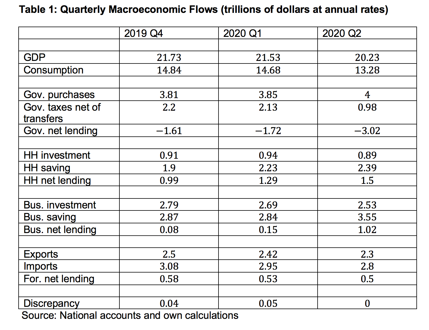
Total profits during the first quarter of this year were $4.18 trillion at an annual rate. To get to business saving or undistributed profits one must subtract direct taxes, interest, dividends, and minor items. The resulting saving estimate is 2.84 (omitting the dollar sign and “trillion” for simplicity). With investment at 2.69, business net lending was 0.15 or 0.7% of GDP of 21.5 (in the range illustrated in Figure 1).
What about the second quarter? The foregoing calculations suggest that corporate profits may rise to 4.89, and saving to 3.55. Investment is not likely to decrease by 30% as in 2009-10. The OECD suggests a drop of eight percent over 2020. Suppose that the decrease in the second quarter is a bit more than ten percent, giving an investment level of 2.53. Business net lending would be 1.02 or five percent of GDP (assuming that it falls by six percent over the quarter). If the government’s debit item is in the range of three trillion it will have to find most funding somewhere else. That basically means households.
Household net lending, government net borrowing
Before getting into details on households, note that exports and imports might drop by (say) five percent each, leading to a second quarter foreign deficit of 0.5, or 2.5% of GDP. “Required” household net lending to meet governing borrowing would then have to be in the range of $1.5 trillion. An illustration appears in Table 1, based on consistent accounts. The numbers are constructed to show how double entry macroeconomic bookkeeping might hang together.
The entries for business and the rest of the world have been described. Household net lending in the second quarter would be 1.5 (trillion dollars) if the sector’s net investment is fairly stable and saving continues its upward trend. Along with our postulated six percent GDP loss, household consumption would fall by seven percent in the second quarter.
In the government accounts, purchases of goods and services for consumption and investment (or “G”) are assumed to increase slightly. A fiscal net borrowing flow of 0.98 emerges if taxes minus transfers decrease from 2.13 to 0.98 trillion dollars. The main goal of CARES and earlier packages is to funnel money via the financial sector to households and business. That is why fiscal transfers increase by over a trillion dollars (six percent of GDP) as an offset to taxes.
Which households provide net lending?
In standard economic data as reported by Taylor with Ömer (2020), spending by the poorest tier of households (say the bottom sixty percent) exceeds their income. That is, in consumer budget surveys they report negative saving. Their income comes roughly half-and-half from wages and government transfers.
”Middle class” households in the 61st to 99th percentiles of the size distribution get 85% of their income from working; the rest comes from rents, proprietors’ incomes, depreciation, and transfers from the government and business. They consume less than they receive, roughly offsetting the negative saving by households with lower incomes.
The top one percent get relatively large labor payments, but almost three-quarters of their income (fifteen times as high per household as the middle class’s) comes from other sources. They also rake in around 70% of capital gains which do not figure in the national accounts. With capital gains, they save around half their income. In other words, most of the household savings flows in Table 1 come from the top one percent and most of their income comes from distributed profits and capital gains. These connections will outlast the pandemic.
Flows, stocks, and the pandemic
Table 1 focuses on flows of money through the financial system. Profits and wages are created by production and distributed across business, households, government, and the rest of the world. Changes in output, employment, external balance, and prices are mediated by these flows.
Flows cumulate into stocks of financial claims which enter portfolios of the various actors. The flow-to-stock transition takes time to build, while financial stocks by themselves can be switched among portfolios in nanoseconds. To an extent, anti-pandemic interventions have taken the form of financial engineering, magicking offsetting financial assets and liabilities into existence to stimulate the real economy. How well these moves will work out remains to be seen but they will generate substantial fees for finance.
Table 1 shows how the pandemic hits pre-existing income inequality. The profit surge is passed to high income households who are free to engage in financial transactions, trading government bonds for other claims as they see fit. Maybe people with low incomes will regain jobs and garner some inflows, but the true beneficiaries will be households bringing in two million as opposed to twenty thousand per year. The government’s attack on COVID ultimately creates wealth in the form of Treasury bonds for households at the top.
Further observations
In June, new COVID-19 hot spots appeared and excess mortality did not abate. Another stimulus package could well be on the way. If it takes the form of a trillion dollar transfer to households, for example, then Table 1 shows that such payments would equal the tax take of the consolidated government sector. Net borrowing would rise to one-fifth of GDP.
Such rapid debt accumulation opens several possibilities. The usual expectation is that government debt is “riskless.”[7] If that holds, then balance sheets of both business and rich households would be substantially stronger after the fiscal expansion. Hyman Minsky (1982) thought that similarly strong private sector balance sheets coming out of WWII were a foundation for the subsequent Golden Age of economic growth. Pandemic-based fear for the economy’s future could undermine the idea that government debt is secure. If that expectation fails, there could be an international portfolio shift against dollar liabilities (irrelevant after the War). Depending on the Fed’s response, there are two possible reactions or a combination. The interest rate could rise, increasing the government’s debt service burden and possibly reducing aggregate demand. Or there could be dollar depreciation, which could be inflationary (see below) and would reduce the external deficit.
Then there is the stock market. In financial jargon, beginning in the mid-1980s successive Governors of the Federal Reserve engineered a Greenspan-Bernanke-Yellen-Powell “put,” utilizing bond market interventions to hold down interest rates. Prices of assets such as corporate shares should roughly equal the market’s expectation about their returns “capitalized” (or divided by) the real interest rate (Taylor with Ömer, 2020). Robust corporate profits should therefore generate high equity valuations if expectation is stable. Today it is anything but stable, if market fluctuations since the pandemic erupted are to be believed. Repercussions on the Dow-Jones or S&P of high profits remain to be seen. A COVID crash if expectation falters is by no means impossible.
Controlled interest rates may also be associated with inflation of goods and service prices, a combination nowadays called “financial repression” by mainstream economists. Inflation has the handy side effect of erasing the real value of debt outstanding, just one aspect of its fundamental social role as a mechanism to redistribute wealth and income.[8] A necessary condition for inflation to take off would be an escalation of labor militancy. Prices cannot spiral in a dynamic process unless they are propelled by steadily rising money wages. Across business cycles the wage share has been trending downward for 50 years. The trend could conceivably be reversed if the pandemic spurs rising demands for worker pay.
Or wage repression and austerity policies could be cemented into place. Almost eighty years ago, in a remarkable paper, Kalecki (1943) pointed out that while in a crisis business interests might support public intervention to create jobs, they would oppose maintaining full employment for fear of losing social and political control. “The sack” may not be required under COVID, but it could be reinstated if need be.
Doubts about the security of holding government debt, a stock market crash, wage-driven inflation, and renewed labor repression are known possible responses to the pandemic. Unknown unknowns may lurk in the future as well.
Appendix
Let X stand for output and L for employment. Between levels X_0 at the beginning of the quarter and X_1 at the end, the growth rate ( X) ̂ of X (for example) is given by
X_1=(1+X ̂)X_0 .
Labor productivity is simply ξ=X⁄L. An exact expression for its growth rate from time zero to time one is
ξ ̂=((X ̂-L ̂))⁄((1+L ̂)) .
Effects of the “interaction term” 1⁄((1+L ̂)) are discussed in the text.
The profit share is a bit more complicated. If π and ψ are shares of profits and wages in factor payments, one has π+ψ=1 and ψ=ω⁄ξ with ω as the real wage. With π_0<ψ_0 there is a boost from negative growth of the wage share to positive growth of the profit share,
π ̂=(-ψ_0 ψ ̂)⁄π_0 =((ψ_0⁄(π_0)(ξ ̂-ω ̂)))⁄((1+ξ ̂)) .
Taking into account the interaction term, the profit share growth rate scales to the difference between productivity and wage growth rates according to ψ_0⁄(π_0 (1+ξ ̂)).
References
Board of Governors of the Federal Reserve (2020) “Consumer Credit – G19” https://www.federalreserve.gov/releases/g19/current/default.htm
Bureau of Labor Statistics (2020) “Employment Situation Summary,” https://www.bls.gov/news.release/empsit.nr0.htm
Federal Reserve Bank of New York (2020) “Jun 05, 2020: New York Fed Staff Nowcast,” https://www.newyorkfed.org/research/policy/nowcast
Kalecki, Michal (1943) “Political Aspects of Full Employment,” Political Quarterly, 14: 332-331
Keynes, John Maynard (1936) The General Theory of Employment, Interest, and Money, London: Macmillan
Minsky, Hyman P. (1982) Can “It” Happen Again?, Armonk NY: M. E. Sharpe
Organization for Economic Cooperation and Development (2020) “OECD Economic Outlook Volume 2020 Issue 1: Preliminary Version,” https://www.oecd-ilibrary.org/sites/0d1d1e2e-en/index.html?itemId=/content/publication/0d1d1e2e-en
Taylor, Lance (2010) Maynard’s Revenge, Cambridge MA: Harvard University Press
Taylor, Lance (2020) “CARES Will Care for Wall Street and Big Business, For Macroeconomic Balance Maybe Not So Much,” https://www.ineteconomics.org/perspectives/blog/cares-will-care-for-wall-street-and-big-business-for-macroeconomic-balance-maybe-not-so-much
Taylor, Lance, and Özlem Ömer (2018) “Where Do Profits and Jobs Come From? Employment and Distribution in the US Economy” https://www.ineteconomics.org/uploads/papers/WP_72-Taylor-and-Omer-April-8.pdf
Taylor, Lance with Özlem Ömer (2020) Inequality from Reagan to Trump: Market Power, Wage Repression, Asset Price Inflation, and Industrial Decline, New York: Cambridge University Press
[1] See Board of Governors of the Federal Reserve (2020).
[2] For example, see the “nowcast” by the New York Federal Reserve (2020). Its annual yearly GDP loss of over twenty-odd percent translates into six percent per quarter. The OECD (2020) predicts a seven to eight percent real GDP loss during this year. The “central tendency” in a range of June 10 Federal Reserve estimates is between -5.5% and -7.6%. See https://www.federalreserve.gov/newsevents/pressreleases/monetary20200610b.htm
[3] Data from Bureau of Labor Statistics (2020).
[4] See https://www.bea.gov/sites/default/files/2020-05/gdp1q20_2nd_0.pdf
[5] Taylor with Ömer (2020) presents a long recital.
[6] Recall a theorem from sixth grade arithmetic stating that a negative number minus a more negative number equals a positive.
[7] In the General Theory word of Keynes (1936) “expectation” means a market consensus, not the standard interpretation in the literature as the first moment of a hypothetical probability distribution of business profits.
[8] Annual inflation rates ranged toward 15% during and after both WWI and WWII, for example, eroding the real value of government debt.
Thanks to INET for support and to Michalis Nikiforos and Thomas Ferguson for helpful discussions.
